Some low discrepancy noise functions

This post is about an attempt to generate blue noise at a point: no state, no offline training, just arithmetic on an index. Honestly I don’t have a good reason for wanting this but it’s probably been at the back of my mind for like 2 years–it just seemed like it ought to be possible. It turns out to be doable in 1D and with a little lookup table we can push it to 2D.

The kind of blue noise we’re going to get is the classic “3dB per octave"¹ blue noise, which might turn out to be not all that useful, who knows. But it will also be low discrepancy, and the tricks in this post to keep it that way all the way to 2D are pretty cool I think. The plan is to take a sequence we already know has good discrepancy, whiten its frequency spectrum, and then turn that into blue noise.

Motivating example: dither

So: low discrepancy blue noise. Breaking that down:

• Low discrepancy: values the noise takes on are evenly spread out. Read on a bit if this is unclear.
• Blue: no or little low frequencies in the noise’s frequency spectrum.
• Noise: unpredictable.

A problem I had writing this post is that it’s not obvious why you’d even want noise with these properties, and the technical answer–reduce variance–is a bit mystifying. This was a good excuse for me to look at dithering a bit more closely. Bart Wronski has a nice series of posts on dither if it’s new to you, but hopefully you can follow this either way.

Here, we want to represent a 64x64 gray square, with a gray value of $0.5$, using only black and white pixels. If we know ahead of time that it is solid gray, we could use a checkerboard pattern as a way to approximate “gray”. But suppose we don’t, and we decide to choose whether to make a pixel black or white by drawing a random value in $[0,1)$ and comparing it to the source pixel; if the random value is less, black, if it’s greater, white. Since we’re using random values, we can do this multiple times and get a different dither pattern every time. Using some functions I’ll get into below, we get this.

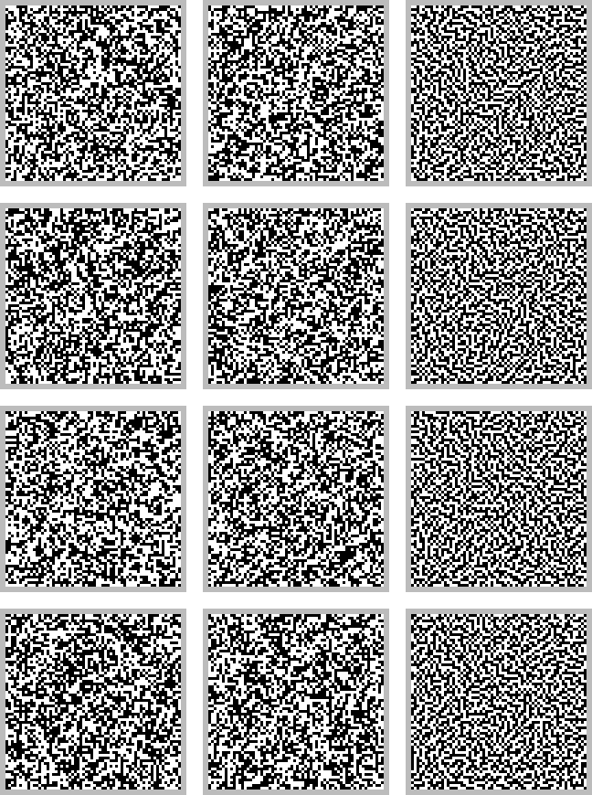
The PRNG is quite bad. By bad I mean like, to my eye, the third square seems to have too many white pixels. So, yes, it will give 1:1 white and black pixels on average, but that’s averaged over all the dithering you could ever do. That’s the problem: we don’t care about the quality of unrealized dither.

The middle column, maybe you can convince yourself it looks different, I dunno. It’s subtle. If you take it upon yourself to count number of white pixels you’ll find that very close to half of them are white, in all four squares. That’s low discrepancy. The noise values we got covered $[0,1)$ much more evenly than random noise. This gives us frequencies of black and white pixels that are always close to the frequencies of the dither we know would be ideal for solid gray.

However, that’s not true over the entire square; there are clumps of black pixels and clumps of white pixels. That’s what blue noise addresses. Which you can see just looking at it, right. This gives spatial frequencies of black and white pixels that better match the ideal dither.

That’s two different kinds of frequency–one in the histogram sense and another in the spectrum sense. I don’t quite know how independent they are. On the one hand, once you have some noise values, you can just rearrange them to get different frequency spectrums with the same discrepancy. On the other, if you want the noise to be low discrepancy ‘everywhere’, without any rearrangement, that rules out long lasting low frequency content. What you’ll find is the more samples you are willing to wait around for until a given run of draws becomes low discrepancy, the more freedom in shaping the spectrum you’ll have. Noise that is low discrepancy everywhere and at all scales has to be blue, though, I think.

Back to the 64x64 squares. Generating a thousand each, the standard deviation of the number of white pixels in a random PRNG square is 32 (!). It’s less than 1 for both the low discrepancy versions. Counting just the top left quarter, at 32x32, it becomes 16, 12, and 2, for the PRNG, white and blue noise respectively. That’s what reducing variance means.

Background

The API that I want is a counter hash, so a function that takes in an index, hashes it, and spits out a noise value at that index. No state carries forward from index to index, every value is computed independently. Like this:

// integer index to 0.32 fixed point
uint32_t noise(uint32_t index);

// usage
for (uint32_t i = 0; i < 512; i++) {
	// convert the noise to a float in [0, 1)
	float x = (float)noise(i) * 1.0p-32f;
	
	// ... do something with x
}

We’re going to follow Practical Hash-based Owen Scrambling by taking a sequence we already know is low discrepancy and shuffling it. We’ll need the nested uniform scramble from that paper, too. As for the sequence, the golden ratio sequence is very easy to compute in the form I want, so we’ll use that.

import np
i32 = np.int32
u32 = np.uint32 

def golden_ratio_sequence(i: u32) -> u32:
	return u32(i) * u32(2654435769) # 0.618... in 0.32 fixed point

def reverse_bits32(x: u32) -> u32:
    x = u32(x)
    x = ((x >> u32(1)) & u32(0x55555555)) | ((x & u32(0x55555555)) << u32(1))
    x = ((x >> u32(2)) & u32(0x33333333)) | ((x & u32(0x33333333)) << u32(2))
    x = ((x >> u32(4)) & u32(0x0F0F0F0F)) | ((x & u32(0x0F0F0F0F)) << u32(4))
    x = ((x >> u32(8)) & u32(0x00FF00FF)) | ((x & u32(0x00FF00FF)) << u32(8))
    x = ( x >> u32(16)                  ) | ( x                    << u32(16))
    return x

def nested_uniform_scramble(x: u32) -> u32:
    x = reverse_bits32(x)
    x ^= x * u32(0x6c50b47c)
    x ^= x * u32(0xb82f1e52)
    x ^= x * u32(0xc7afe638)
    x ^= x * u32(0x8d22f6e6)
    return reverse_bits32(x)

def okay_blue_noise(i: u32) -> u32:
	return golden_ratio_sequence(nested_uniform_scramble(i))

You can get a reordering of any sequence you like by hashing the index with nested uniforms scramble.

It’s a bit intimidating, but the important thing about it is each hex constant there is an even number. In binary, multiplying by an even number sends bits to the left, so each xor permutes bits in a low-to-high direction. The authors wanted to permute bits high-to-low, and so reverse the bit order before and after. So, it’s a hash, where the action of each bit on the hash is constrained to only permute bits below itself. And the xors are invertible, meaning each input maps to a unique output.

A consequence of this that can give you some intuition for what it does is that the high bit of the input is always preserved. So, as a counter hash, the first $2^n$ inputs map to u32s below $2^n$. And since you know that holds for $2^{n+1}$ as well, you also get that $[2^n, 2^{n+1}]$ maps to $[2^n, 2^{n+1}]$. In these intervals, the shuffled sequence produces the same values as the underlying sequence, just in a different order. This doesn’t fully explain its behaviour as a hash but it’s enough for us to get going with.

By the way, you can also think of the (fixed point) golden ratio sequence as a shuffle of the integers in u32. They all appear exactly once.

This has all been background, but before we get to the good stuff, let’s look at what we have:

import matplotlib.pyplot as plt
plt.rcParams['figure.figsize'] = (9,2)

def spectrum(seq):
    S = np.fft.rfft(2 * seq - 1.0)
    return np.abs(S) / len(seq)

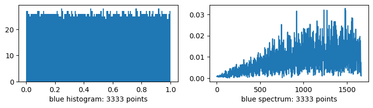
def plots(name: str, seq_u32):
    seq = seq_u32 * np.ldexp(1, -32)

    figure, (histogram_axis, spectrum_axis) = plt.subplots(1, 2)

    histogram_axis.hist(seq, 128)
    histogram_axis.set_xlabel(f"{name} histogram: {len(seq)} points")

    dft = spectrum(seq)
    spectrum_axis.plot(dft)
    spectrum_axis.set_xlabel(f"{name} spectrum: {len(seq)} points")

n = 3333

Bad histogram…

from numpy.random import default_rng
rng = default_rng()
plots("PRNG", rng.integers(0, 0x1_0000_0000, size=n))

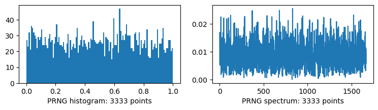
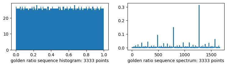
Bad spectrum…

i = np.arange(n)
plots("golden ratio sequence", golden_ratio_sequence(i))

Noise with a flat histogram?

plots("nested uniform scramble-shuffled grs", okay_blue_noise(i))

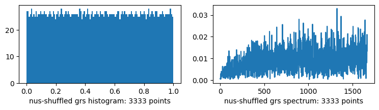
This already has some low frequency attenuation. Well, if you drop the last bit reversal step and the golden ratio sequence and instead use it directly, not as a shuffle, it comes out even better. But my plan here is to clear the way by getting to white noise, and to use that as a base for more noise colours, so forget I said anything.²

Xorshift

We need more unpredictability. To that end, let’s look at using xorshift as a counter hash. Specifically, lets look at the low bits.

def xorshift(x: u32) -> u32:
    x = u32(x)
    x ^= x << u32(13)
    x ^= x >> u32(17)
    x ^= x << u32(5)
    return x

i = np.arange(16)
print(i)
print(xorshift(i) & 0b1111)

[ 0 1 2 3 4 5 6 7 8 9 10 11 12 13 14 15]
[ 0 1 2 3 4 5 6 7 8 9 10 11 12 13 14 15]

Uh, hold on,

xorshift(i + 64 + 16) & 0b1111

[ 5 4 7 6 1 0 3 2 13 12 15 14 9 8 11 10]

The lower 4 bits are a (not very random) permutation of the original 4-bit sequence!! The Xorshift* variants preserve this property and is at least superficially random-looking so let’s use that instead from now on (constant from Melissa O’Neill):

def xorshift_star(x: u32) -> u32:
    x = u32(x)
    x ^= x << u32(13)
    x ^= x >> u32(17)
    x ^= x << u32(5) 
    x *= u32(0x9e02ad0d)
    return x

xorshift_star(i + 64 + 16) & 0b1111

[ 1  4 11 14 13  0  7 10  9 12  3  6  5  8 15  2]

This works for powers of two up to $2^{16}$. This isn’t a good way of generating permutations–it can’t make all that many–but we don’t need it to be good. LCGs work this way, too.

Now, because of this we can bestow xorshift with the high-bit-preserving property³ of nested uniform scramble by fixing the high bit and masking off any new bits placed above it. And we know that when we do this, every input still maps to a unique output, so long as we only scramble the lower 2 bytes. Using all 16 bits is way too random, so we can cap the number of bits we allow to be scrambled this way, and use the rest as a seed that selects a permutation. Looks like this:

def all_ones_below_high_bit(x: u32) -> u32:
    x = u32(x)
    x |= (x >> u32(16))
    x |= (x >> u32(8))
    x |= (x >> u32(4))
    x |= (x >> u32(2))
    x |= (x >> u32(1))
    # this last shift: the high bit is not included
    return x >> u32(1)

def unfolded_masked_xorshift(x: u32, cap_mask: u32) -> u32:
    mask = all_ones_below_high_bit(x & cap_mask)
    upper = x & ~mask
    lower = xorshift_star(x) & mask
    result = upper + lower
    return result

Every bit we include in this scramble increases discrepancy–bits can permute bits to their left, here. We can claw back a bit by treating the high bit of cap_mask as a kind of sign bit and flipping all this logic to work backwards when its set.

def masked_xorshift(x: u32, bits: u32 = 8) -> u32:
	# all ones if (x & 0x100) == 0x100, all zeros otherwise
    sign_mask = i32(x << u32(31 - bits)) >> i32(31)
    sign_mask = u32(sign_mask)
    cap_mask = u32((1 << bits) - 1)
    return unfolded_masked_xorshift(x ^ sign_mask, cap_mask) ^ sign_mask

This is all pretty abstract. You can see what it does by plotting the difference with its input:

i = np.arange(1024)
plt.plot(i - masked_xorshift(i))

As a shuffle, this shows you where elements are being moved to, relative to their original position. With bits = 8, that distance is never more than 128. So, while this scramble doesn’t have all the nice properties of nested uniform scramble, we do get a version of the $[2^n, 2^{n+1}]$ bijection property that repeats inside every chunk of size 256. So discrepancy-wise it’s kind of bad, but we can bound the bad with bits.

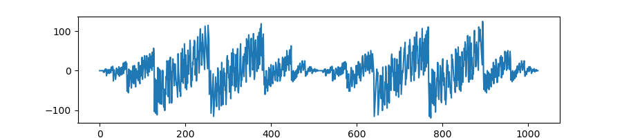
Now we’ve got low discrepancy white noise:

def white_shuffle(i: u32) -> u32:
    s = i
    s = masked_xorshift(s)
    s = nested_uniform_scramble(s)
    return s 

def white(i: u32) -> u32:
    return golden_ratio_sequence(white_shuffle(i))

i = np.arange(3333)
plots("white", white(i))

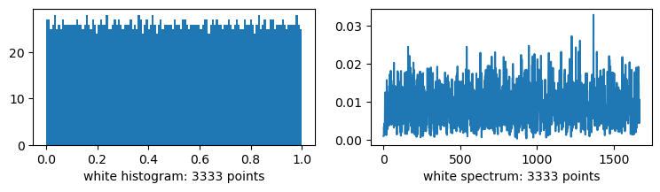
Look closely at the lowest frequencies of the spectrum. There is a slight gradient away from zero. This is what bits controls: the slope of that gradient. I found that at 11 bits it’s qualitatively pure white noise with no obvious correlations (… aside from an usually flat histogram). But it’s just too much random. For example, the variance in the dither example really suffers. And variance is what we care about.

Next: gotta eyeball it in 2D. You gotta.

plt.rcParams['image.cmap'] = 'gray'
plt.rcParams['image.interpolation'] = 'none'
px = 1/plt.rcParams['figure.dpi']

n = 512
i = np.arange(n*n)
f, ax = plt.subplots(figsize=(n*px, n*px)); ax.axis('off')

ax.imshow(white(i).reshape((n,n)) * np.ldexp(1, -32))

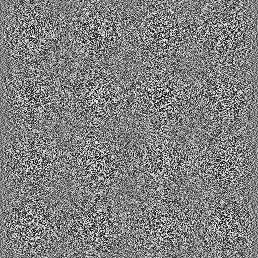
Ah. The edges. It’s bad. Okay, that’s our choice of bits. It’s too small. But we don’t have to increase bits, we can get away with doing another nested uniform scramble. This is kind of painful on x64, where bit reversal spews instructions everywhere, but, eh. There’s a trade-off between performance and discrepancy here and I completely lack any insight on it.

def white_shuffle(i: u32) -> u32:
    s = i
    s = nested_uniform_scramble(s)
    s = masked_xorshift(s)
    s = nested_uniform_scramble(s)
    return s 

f, ax = plt.subplots(figsize=(n*px, n*px)); ax.axis('off')
ax.imshow(white(i).reshape((n,n)) * np.ldexp(1, -32))

👍

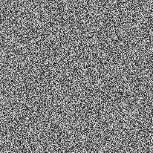
Blue noise

Now, to transmute this into blue noise. Filtering the noise directly destroys low discrepancy, so no perfectly tuned cut off frequency and ripple here. But I think what I’m about to suggest might seem to come out of nowhere for some people. With that in mind, here’s what I was thinking about when I realised this: the unshuffled golden ratio sequence has the property that

golden_ratio_sequence(i * -1) == 1 - golden_ratio_sequence(i)

In other words, you can go backwards from zero, and it’s the same, just inverted around $0.5$. So what if we interleaved the forwards sequence with the backwards sequence? The two sequences would meet in the middle. Seems natural, right?

This turns out to do something very specific in the frequency domain: it fills in the new frequency bins–twice as many samples, twice as many bins–with a copy of the frequency spectrum then high pass filters the whole thing. This is entirely due to the right hand side of the above equation, so when we use that form, it also works on the shuffled sequence.

But why!? If you’re comfortable with DSP this can be hand-waved as being the composition of three steps: zero-stuffing to repeat the frequency spectrum⁴, applying the simple low-pass filter $[1, 1]$, and then reversing the frequency spectrum by inverting every second sample. This turns the low-pass filter we just applied into a high-pass filter.

Even so, that last bit might need more explaining if you haven’t seen it before. This is directed at DSP people (don’t worry about it). First, in this context, $1 - a_i=-1\cdot a_i,$ because in 0.32 fixed point, we have 0x1_0000_0000 - a[i] = 0 - a[i]. From this we get that inverting every second sample is equivalent to point-wise multiplication by the signal

$x[n] = ...-1,1,-1,1... = e^{i\pi n}$

which is your frequency shift in the time domain⁵ operator set to $\pi$, a half turn. This places all the negative frequencies into the positive part of spectrum, and because of the conjugate symmetry of real signal DFTs, they are the mirror image of the positive frequencies.

DSP talk’s over. Intuitively, something like this should happen–low frequencies are slow movement, high frequencies are rapid movement. Forcing the sequence to repeatedly jump from one half to the other pushes all the frequencies higher.

For ‘noise’ this has the weird property that every second value is just the previous value flipped around $0.5$. A gray code round can get rid of that–rightward invertible action of the bits like before by the way, this is a scramble. Shift here is by 6 because reserving the high bits preserves the frequency spectrum. That’s where all the energy in the signal is.

def kronecker_sequence(i: u32, a: u32) -> u32:
    return u32(i) * u32(a)

def blue(i: u32) -> u32:
    s = white_shuffle(i >> 1)
    b = kronecker_sequence(s, 2654435770) # 0.31 fixed point golden ratio
    odd = u32(i & 1)
    b ^= (odd ^ u32(1)) - u32(1);         # negate on odd indices
    b += odd           
    b ^= b >> u32(6)                      # gray code round
    return b

i = np.arange(3333)
plots("blue", blue(i))

Observations without narrative flow

We can get red noise by not doing the inversion step. This duplicates every element, which is bad, but we can scramble every odd element. (Technically, scrambling is a thing you do to the values of a low discrepancy sequence, and shuffling a thing a thing you do to their indexes. In fixed point they are kind of duals to one another, at least when you have a proper scramble, like nested uniform scramble is.) This raises the spectre of a scrambled odd value colliding with an unscrambled even value. None of this is ideal from a discrepancy point of view, but whatever.

There is another purely real rotation we can do: a quarter turn of the frequency spectrum, using $e^{i\pi n/2} = \ldots -1,0,1,0,-1,0,1 \ldots$You can fill in the zeros with another sequence generated with another shuffled Kronecker sequence. Martin Robert’s R2 works well. A quarter turn of red noise and a quarter turn of blue noise gets you green? and.. violet? I guess? noise? With the middle frequencies band-passed or cut. Unfortunately, it doesn’t extend to 2D using the technique I’m about to describe so I’m dropping it here. That it doesn’t work is interesting in its own right, I suppose.

blue doesn’t have equidistribution. That is, some inputs map to the same output. 0 appears twice and who knows about 0x8000_0000. But it’s also lost an entire bit in the interleaving of two sequences. These are both length $2^{32}$ and they interleave to a sequence of length $2^{33}$. We only have 32 bits to index it with. Rounding the constants to have a zero bit in the last place (and a one bit in the second last place) gives us a pair of sequences of length $2^{31}$. Now every value before the gray code round is even, but we know exactly what values we’re missing, the odd values, and what values we are double counting, the even values. I’m not bothered about that low bit, because we’re going to round it away anyway on conversion to float, and if you want integers, the high bits are better.

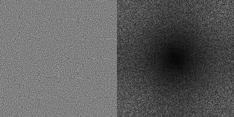
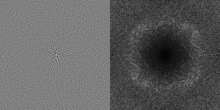
2D blue noise

Dumping it out in 2D doesn’t work, but the way it doesn’t work is instructive so let’s look at it.

def spectrum_2d(img):
    dft = np.abs(np.fft.fftshift(np.fft.fft2(img)))
    dft /= dft.shape[0]
    return np.clip(dft, 0, 1)

def lookit(image):
    f, ax = plt.subplots(figsize=(2*image.shape[0]*px, image.shape[1]*px))
    ax.axis('off')
    ax.imshow(np.hstack((image, spectrum_2d(image))))

n = 384
i = np.arange(n*n).reshape((n,n))
noise = blue(i) * np.ldexp(1, -32)
lookit(noise)

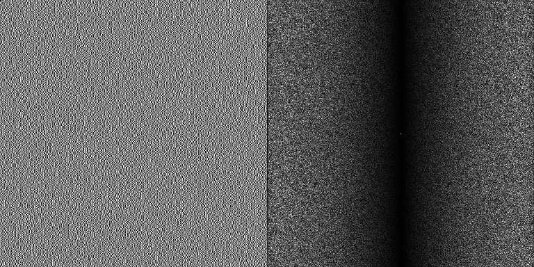
It’s blue horizontally, but in no other direction. Okay. At this point, we can generate another noise image, transpose it so it’s blue vertically, and drop it on top, like

noise[x,y] + more_noise[y,x]

and yeah it works but the spectrum isn’t that good and the triangle distribution you get out of the sum isn’t all that low-discrepancy either. If you don’t care about discrepancy, you could use some cheap PRNG here instead of low discrepancy noise and filter this right in a shader. Since you could design the filter to smooth out some of the anisotropy this method has, I think it could be pretty good.

But to preserve low discrepancy we can decide that the issue is the path the noise takes over the image, and so let’s find a better path. I tried to find a way to do this with just arithmetic, and I got nowhere. But I did find a path that works that’s easy to compute offline, and it turns out we can tile the path. So this might be an okay compromise.

No imaginative thinking here, horizontal path bad circular path good. This bins pixels into concentric rings, then pixels within each ring are sorted by their angle.

def spiral(n: u32, lo: float, hi: float):
    x, y = np.meshgrid(np.linspace(lo, hi, n), np.linspace(lo, hi, n))
    # two sqrts: one for the distance, two to adjust for spirals closer to
    # the origin being tighter (think random sampling in a circle)
    xy = np.round(np.sqrt(np.sqrt(x*x + y*y)) * np.sqrt(n*n + n*n))
    # rescaled to a reasonable range that makes debugging possible without
    # a third eye
    angles = (np.arctan2(y, x) + np.pi) / (2 * np.pi)
    # sort by magnitudes then angles (I don't know why lexsort is
    # little-endian), then invert the sort
    spiral = np.lexsort((angles.flatten(), xy.flatten())).argsort()
    return spiral.reshape((n,n))

s = spiral(n, -1.0, 1.0)
noise = blue(s) * np.ldexp(1, -32)
lookit(noise)

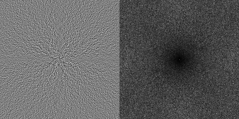
… looks weird. Something to do with the origin. Don’t wanna think about it.

s = spiral(n, 2.0, 4.0)
noise = blue(s) * np.ldexp(1, -32)
lookit(noise)

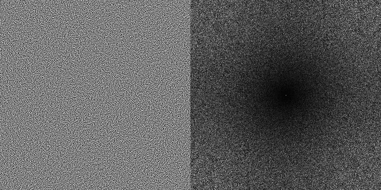
Nice. One reason this path is hard to replicate/approximate using only arithmetic on x and y is that it wraps at the edges in a nice symmetry breaking way that I don’t really understand:

spiral(8, 2.0, 4.0)

[[ 0  2  1  6 10 20 19 32]
 [ 4  3  7 12 11 21 34 33]
 [ 5  8 14 13 23 22 35 47]
 [ 9 16 15 25 24 37 36 48]
 [18 17 27 26 39 38 49 56]
 [30 29 28 41 40 51 50 57]
 [31 44 43 42 53 52 59 58]
 [46 45 55 54 62 61 60 63]]

And here it is with a 64x64 path, tiled using the z-order curve:

def left_shift_2(x: u32) -> u32:
    x = (x ^ (x << 16)) & 0x0000ffff
    x = (x ^ (x << 8)) & 0x00ff00ff
    x = (x ^ (x << 4)) & 0x0f0f0f0f
    x = (x ^ (x << 2)) & 0x33333333
    x = (x ^ (x << 1)) & 0x55555555
    return u32(x)

def z_order(x: u32, y: u32) -> u32:
	return left_shift_2(x) + (left_shift_2(y) << u32(1))

tile_bits = 6
tile_n = 1 << tile_bits
tile_mask = tile_n - 1
tile_path = spiral(tile_n, 2.0, 4.0)

def blue_2d(x: u32, y: u32) -> u32:
    x_lo = x & tile_mask
    y_lo = y & tile_mask
    x_hi = x >> tile_bits
    y_hi = y >> tile_bits
    tile = z_order(x_hi, y_hi)
    i = (tile << u32(2*tile_bits)) + tile_path[y_lo, x_lo]
    return blue(i)

x, y = np.meshgrid(np.arange(n), np.arange(n))
noise = blue_2d(x, y) * np.ldexp(1, -32)
lookit(noise)

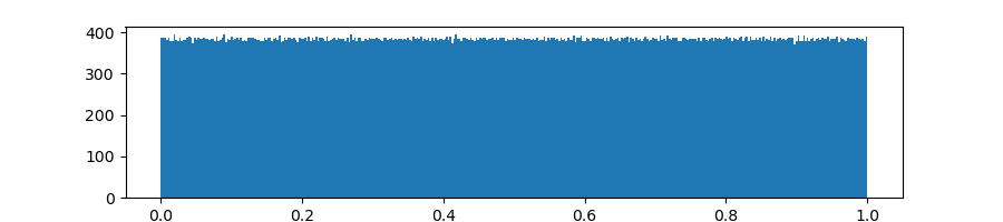
Histogram’s still good:

plt.hist(noise.flatten(), 384)

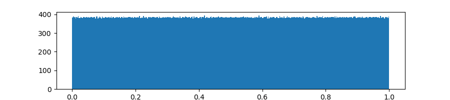
So that’s a 8KB lookup table that’s good for as much noise as you can index with an integer, and you can always get more constants to replace the golden ratio with if you need more. (I’m not super satisfied with this, I wanted 0KB). Also some tiling artifacts where there is a too consistent lack of correlation between adjacent pixels at tile boundaries, which is weird to think about. If you didn’t see it forget I said anything!!

Part of the reason this works at all is that the quality of the noise that we’re threading through the image is not, spectrum-wise, all that good. With better noise, not only do you see the tiling clearly, the spectrum is really no better–it’s determined by the spiral function in a way I don’t understand. So I’m not sure if this could be extended to 3D with just a path. But even if it does, for higher dimensions I doubt it would work all that well without huge lookup tables, because as the number of dimensions goes up the number of edge voxels increase faster than the number of interior voxels.

Dither revisited

Since we started with dither, here’s some real dither. Usually for dither you want triangular noise rather than uniform. Triangular refers to the shape of the histogram. Alan Wolfe has a nice way of getting a triangle distribution out of uniform noise that perfectly preserves discrepancy, so I’m going to use that. Hastily converted to python:

def uniform_to_triangle_dist(x):
    # From demofox @ https://www.shadertoy.com/view/4t2SDh
    x = (x + 0.5) % 1
    orig = x * 2.0 - 1.0
    nz = orig != 0
    x[~nz] = -1
    x[nz] = orig[nz] / np.sqrt(np.abs(orig[nz]))
    x = x - np.sign(orig) + 0.5
    x = (x - 0.5) * 0.5 + 0.5
    return x

An alternative would be to use R2 to get another noise value to add to the first, you only need an extra multiply after all the shuffling to get it. Yet another alternative would be use more noise offset by half a tile to obscure the tiling artifacts.

Code’s here. Quantized to 4 bits with 2 bits of dither. The top row is a gradient we’re dithering and what you get quantizing without dithering. Then it’s left: uniform noise dither, right: triangle noise dither. And top to bottom: random, this post’s white noise, this post’s blue noise, and last I’ve put known-good void and cluster blue noise.

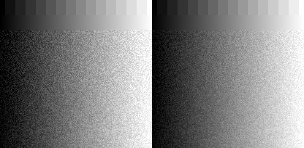
Yup, it dithers 👍 Not as good as a good texture, but that’s okay.

The white noise… I don’t know what I expected.

Bonus

The low bits of the spiral function have a blue spectrum:

s = (spiral(384, -0.08, 0.08) & 7) / 8
lookit(s)

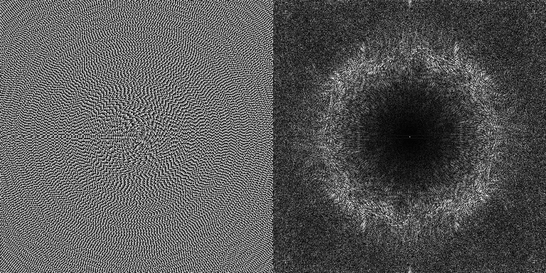
Which suggests maybe we can reverse the bits and get something interesting out?

s = u32(spiral(384, -0.08, 0.08))
s = masked_xorshift(s, 2)
s ^= s >> 1
s = reverse_bits32(s)
s = nested_uniform_scramble(s)
lookit(s / s.max())

Huh. Conceptually, this is just a reordering of pixels–you could replace that divide by a shift to turn it into a true permutation. It’s not noise, though. I tried some things, like rotating some tiles, placing the origin of the spiral at the corners, adding random jitter to the magnitude and angles in spiral, but nothing worked very well at getting rid of the obvious structure while maintaining the spectrum. This is interesting, though.

Bonus 2

I have no idea what is going on here.

def red(i: u32) -> u32:
    s = white_shuffle(i >> 1)
    r = kronecker_sequence(s, 2654435770)  # 0.31 fixed point golden ratio
    r[(i & 1) == 1] ^= r[(i & 1) == 1] >> u32(6)
    return r

def red_2d(x: u32, y: u32) -> u32:
	# note the right shift--this isn't z-order
    i = left_shift_2(x) + (left_shift_2(y) >> u32(1))
    return red(i)

noise = red_2d(x, y) * np.ldexp(1, -32)
lookit(noise)

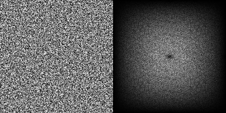
Histogram’s okay, too, but it’s pretty bad within the bins.

plt.hist(noise.flatten(), 384)

Bottom text

Here’s the code for this post without all my words around it.